An Albert Szent-Györgyi Moment for Climate Science

Dr Chris Barnes, Bangor Scientific and Educational Consultants, Wales, UK, LL57 2TW. E-mail doctor.barnes@yahoo.co.uk

Submitted to a peer reviewed journal for publication. Submission date 02/02/2025.

Abstract

The hypothesis that the position of the magnetic North Pole (Dip Pole) (latitude) ought to be very highly correlated with global temperature change on Earth has been tested and shown to be correct. The probability of such a correlation happening by chance is close to zero. Moreover, this has likely been the dominant climate driver for the last 2000 years. Granger causality test shows Pole Shift drives temperature with up to a two-year lag (Figure1). Two new climate models with and without CO₂ are developed and tested. Both models successfully predict modern warming, the Medieval Warm Period (MWP), and the Roman Warm Period (RWP) in time (figures 3+4). The model excluding CO₂ (figure 4) predicts past warming with stronger amplitude. This model also predicts the Little Ice Age ( LIA) with a seamless transition into the Modern Warm Period using the real data sets (figure 5). As Pole swings Northwards, interacting region shifts to higher ionospheric altitudes and combined particle precipitation changes (EEP) reduce albedo, hence increase forcing (figure 2) by virtue of their changes to the world’s clouds, provide calculated values in the region of 81% of recent warming, with the rest (15%) mainly of solar origin. CO₂ at most could contribute 3.9% of all warming. The detail disclosed above represents a profound and crucial discovery for climate science and its future direction. We need no longer try to mitigate so much for CO2, but we will desperately have to understand our geomagnetic climate and possibly how anthropogenic factors such as ELF radio transmitters and power systems and aviation aerosol may also change EEP. Preliminary investigations indicate that because South dip-pole is not antipodal and moves at different rates and in different directions this accounts for different rates of Antarctic warming and Southern Hemisphere Cloud behavoiur also.

Introduction

In 1982, I had the great pleasure of meeting Professor Albert Szent-Györgyi, Nobel Prize winner. I was a young postdoc working on polymer tribo-charging and surface states, and he was a biologist who, even in his twilight years, had an idea that charge transfer complexation involving methyl glyoxal could be relevant in cancer biology. I tested his idea for him. The rest is history and not relevant to a climate science paper, except insofar as Albert was reputed to have said words that make up a now-famous quote: “Understanding is seeing what others have already seen and thinking what no one else has ever thought.” I was not your average postdoc; I never put all my eggs in one basket. I never narrowed my academic field to the point where I wore blinkers to the rest of the world of science. Indeed, after working as a postdoc on three different contracts, I branched out and became a multi-disciplinary scientific consultant, and I also hold patents spanning many disciplines. As a lifelong learner with a keen interest in UK weather since the 1970s, I took it upon myself to learn some climate science. I am not a “climate denier” in the sense that I do not deny that climate changes—indeed, it has always changed—but you can call me a “climate enquirer” as I seek the true causes of change, whether natural or anthropogenic.

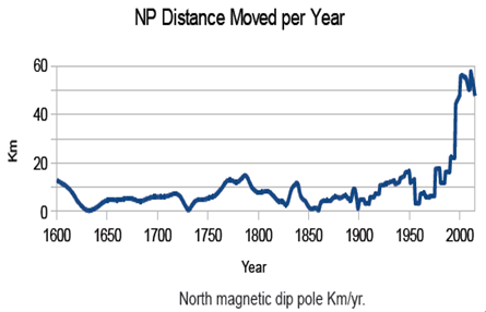
I began writing papers on climate science and weather in 2012 and deposited them on my own website. I always had it uppermost in my mind that there was something fundamentally wrong with the anthropogenic global warming theory, at least with an entire causation by CO₂. I have discussed what I feel are some of the reasons for this elsewhere⁴. Continuing with this in mind, I have always been fascinated by the fact that modern warming commenced in earnest just after the Dalton Minimum (1790–1830), and I was further struck by recent comments that, after the 1970s cooling and the late 1990s to early 2000s hiatus in warming, from 2022 warming appears to have accelerated at an alarming rate and beyond the slope of increase in CO₂ meant to account for it in climate models⁵. I began to ponder other physical factors on this little Earth of ours that had accelerating rates of change. I was struck by the fact that the North Magnetic Dip Pole is moving just so. The drift of the magnetic North Pole from Canada to Siberia has increased from an average rate of 9 kilometres per year until 2000 to about 50–60 kilometres per year afterward. I also noted that, taking in the Maunder and Dalton minima, the magnetic North Pole appeared to move very slowly, remaining in its hitherto most recent set of most south-westerly positions, whereas it has since moved significantly northwards. Hence, an initial inspiration for a testable hypothesis and for the writing of this paper arose.

The writing of this paper has also been inspired by the fact that almost all recent warming can be shown to be due to a fall in Earth’s albedo and changed cloud distributions—see, for example, Goessling et al.⁶, Wu et al.⁷, and especially Nikolov and Zeller⁸. It was further inspired by my 2017 observations of an anthropogenic warming somehow linked to Earth’s power systems, which I have previously ascribed to their influence on the Van Allen Belts and energetic particles, especially electrons but also solar protons⁹. The thought occurred to me that, since the auroral oval is centred around the magnetic North Dip Pole—where field lines are perpendicular to the surface—and not the North Pole per se, any shift in energetic particle interactions brought about either anthropogenically or by movement of the magnetic pole itself ought to change the polar electrojet, the stratospheric polar vortex (SPV), jet streams, and clouds in general, hence also changing the weather and climate.

So, if Earth’s albedo is changing, one needs to look for drivers of those changes. Other than anthropogenic changes, any heating of the planet ought, then, to be down to the Sun or other extraterrestrial sources and/or to changes in features of the solid Earth or oceans. The final piece of inspiration that hit me was to think that maybe there is more to the Sun’s interaction with Earth than its irradiance (TSI), a good measure of solar activity being the 10.7 cm solar flux. I have previously suggested that solar magnetism would be of crucial importance for climate¹⁰.

Hence, bringing all this together and having my “Szent-Györgyi moment,” I thought of the interplanetary magnetic field (IMF) and how it may vary and interact with our wandering magnetic North Pole. Moreover, I thought that not only would the moving North Pole have an IMF/EEP connection, but it would also change Earth’s tilt, sphericity, and rotation—the latter has been known about since the 1950s, see for example Vestine (1953)¹¹—and hence would have an amplification or modulation effect on TSI but also on atmospheric angular momentum pressure, see for example Lam et al. (2013)¹². Thus, I created a hypothesis that the position of the magnetic North Pole ought, perhaps through a combination of these factors, to be very highly correlated with global temperature change on Earth. Bucha (1980)¹³ was possibly the first to investigate tentative correlations between geomagnetic, climatic, and meteorological phenomena, with the object of demonstrating the function of the geomagnetic pole and changes of its position in controlling the climate and weather. It was not until 2009 that Kerton¹⁴ speculated on a possible connection but was still unable to establish the full causes. Goralski (2019)¹⁵ advanced a new climatic theory, explaining how the effects of Earth’s coating movement result in magnetic pole movement. There are also known weak influences of Earth’s field on ocean circulations, but with longer timescales than those considered here¹⁶.

Testing the Hypothesis

When it comes to movements of the geomagnetic North Pole, there are several possibilities to consider for possible correlation with Earth temperature changes. Does one, for instance, consider latitude or longitude or a combination of the two? If the latter, then from where does one take a bearing? Also, the pole movement has been accelerating a lot more of late. Interestingly, so has climate change. Does one need to factor in this acceleration in some way? For instance, the distance moved by the pole per year¹⁷ looks tantalizingly close in form to a plot of modern global warming.

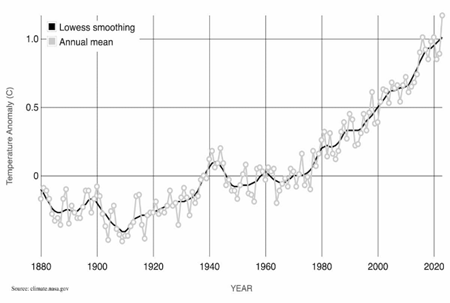
Since the pole has moved both northwards and eastwards since the Dalton Minimum, the first logic I employed was to try plotting its Haversine bearing relative to an arbitrary starting position in 1830. At least this ought to simplify matters and provide a single, testable variable. For temperature, I used the NASA Goddard Institute for Space Studies (GISS) Surface Temperature Analysis (GISTEMP) dataset, v4. For the position of the magnetic North Dip Pole, I used data from the National Geophysical Data Center¹⁸. I constructed the following data table:

Table 1
I plotted the data from Table 1 using Hyams graph plotting suite. Not only was there a near-perfect correlation, but it also accounted for observed hiatuses as well. The plot gave R = 0.993 for the above data, and the two-tailed P-value equals less than 0.0001; by all conventional criteria, this difference is extremely statistically significant. Moreover, this represents some 98.6% of all warming since 1830. As this was a preliminary test, I did not include the residual analysis, but it is easy to see from just the data points that as the motion has increased, so has the linearity and hence the certainty that this is mirroring the main climate driver(s).

I was, however, mindful that this high R-value had been generated from a mere 14 degrees of freedom. I decided to try the same Haversine procedure with a full yearly dataset spanning 1850–2020, hence providing over twelve times as many degrees of freedom. This time the regression was much weaker. I suspected that the dog-leg motion of the pole in the 1800s may be a possible cause, and I considered that EEP interaction would be more likely to be initiated above the auroral oval, which will on average encircle all longitudes at whatever value of latitude it descends to. Thus, I concluded that latitude of the Dip Pole ought to be the most significant variable. I performed a single linear regression of all 170+ points, latitude versus temperature change, and the R-value was considerably higher than for the same temperature data regressed against the Haversine bearing. Also, despite the above trial result suggesting the irrelevance of CO₂, I decided, given recent “consensus,” to include it as an additional X variable and employ multiple linear regression analysis on the same 170+ points using the calculator at https://www.statskingdom.com/410multi_linear_regression.html. The model derived is equation (1), wherein X₁ is the CO₂ concentration in ppm and X₂ is the latitude. The data table for the regressed data is shown in the appendix.

Ŷ = -4.127114 + 0.00529962 X₁ + 0.0320038 X₂ ………………… (1)

Correlation matrix (Pearson)

It can be seen from the correlation matrix that X₂ carries the strongest weight.

1. Y and X relationship: R² equals 0.899546, meaning that the predictors (Xᵢ) explain 90% of the variance of Y. Adjusted R² equals 0.89835. The coefficient of multiple correlation (R) equals 0.948444, indicating a very strong correlation between the predicted data (ŷ) and the observed data (y).

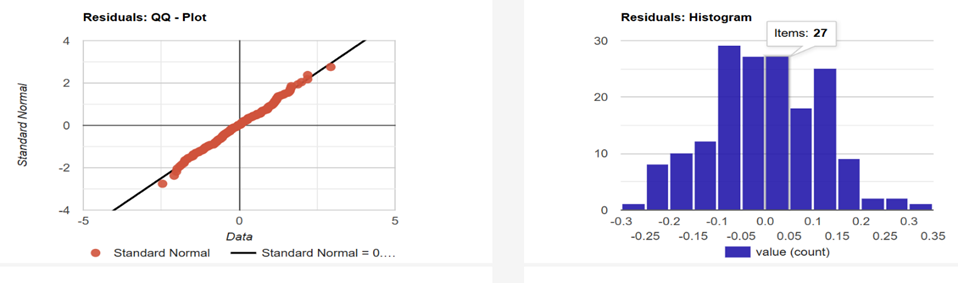
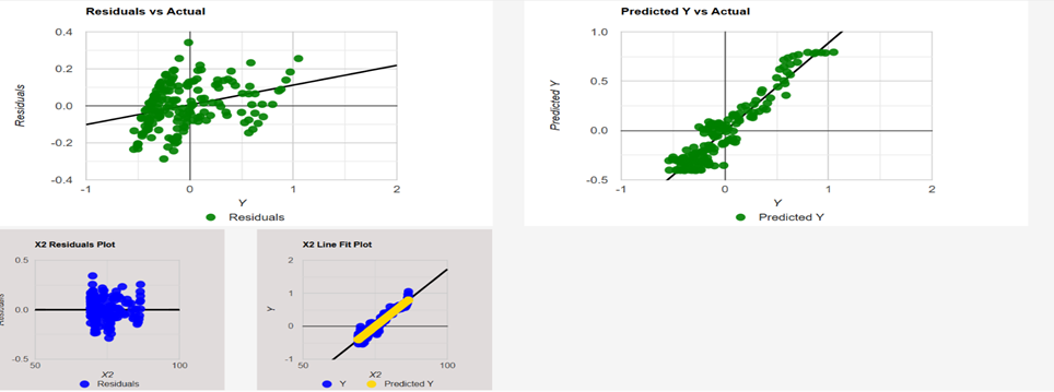
2. Goodness of fit: Overall regression: right-tailed, F(2,168) = 752.206029, p-value = 0. Since p-value < α (0.05), we reject the H₀. The linear regression model, Y = b₀ + b₁X₁ + ... + bₚXₚ + ε, provides a better fit than the model without the independent variables, resulting in Y = b₀ + ε. All the independent variables (Xᵢ) are significant. However, there was a high multicollinearity concern as some of the VIF values are bigger than 10. The multicollinearity may influence the coefficients or the ability to choose the predictors, but not the dependent variable (Y). I will discuss this later when I deal with modelling the Roman and Medieval Warm Periods. The AI calculator suggested removal of X₁ from the model. But before I did so, I investigated the residuals and the climate sensitivity of the two parameters.

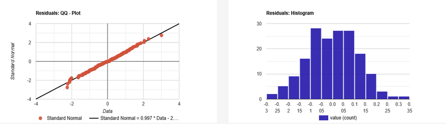
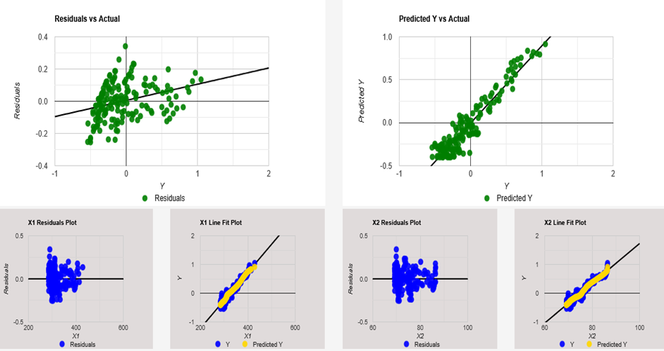
The histogram has a good bell curve, suggestive of real, meaningful data. The X₁ and X₂ residuals are truly fascinating. There is no known physical way in which CO₂ or temperature could drive an internal parameter of the “solid” Earth. However, if pole shift is driving temperature, then it could be driving additional natural CO₂ as well. Alternatively, another parameter related to EEP could be cross correlated with CO₂, and I have remarked on this elsewhere⁹.

Assuming, for the moment, both X variables in the model to be real yields roughly equal climate sensitivity of 34 mK and 32.3 mK per decade for X₁ and X₂, respectively. For CO₂, this represents a further 1.506°C of warming if CO₂ were to double, assuming linearity. However, as I have said before, the reality of CO₂ in the model is questionable, and interestingly, I have previously theorized on simple solar system measurements that showed that the order of warming by CO₂ at present levels in Earth’s atmosphere ought to be of the order of a few milli-Kelvin². Further reinforcing these findings, Qing-Bin Lu (2025)³ finds no recent significant trends in total GHG effect in polar and non-polar regions, respectively. Koutsoyiannis and Kundzewicz (2020)¹⁹ found that for Earth CO₂ concentrations, the dominant direction is that temperature first increases, and then CO₂ concentration follows. Changes in CO₂ follow changes in T by about six months on a monthly scale, or about one year on an annual scale. One interpretation of this result would again be if CO₂ is not a significant driver and that another factor causes temperature rise, as in line with the present discovery perhaps. YoungSeok Hwang et al. (2021)²⁰ found, using satellite measurements, no evidence for a global decrease in CO₂ concentration during the first wave of the COVID-19 pandemic, despite others finding local decreases adjacent to roads, power stations, and factories and the like. One possible conclusion here is that perhaps the warming Earth is generating far more of its own CO₂ to the extent wherein human-generated CO₂ pales to insignificance. On the other hand, Feldman et al. (2015)²¹ claim to have measured the real effect of a CO₂ increase of 22 ppm in the atmosphere, but its arguments have several weaknesses. The limited spatial scope, heavy reliance on radiative transfer models, exclusion of cloud effects, short period, lack of temperature analysis, and potential overstatement of novelty all raise questions about the robustness and broader applicability of those findings. Additionally, the study could be strengthened by addressing alternative explanations and placing the results in a longer historical context. While the paper seeks to add to our understanding of CO₂’s role in Earth’s energy balance, its limitations highlight the need for more comprehensive, globally representative studies to fully validate the magnitude of the link between CO₂ forcing and climate change. Moreover, other recent satellite studies have shown that almost all warming in the last two decades has been due to the disappearance of mid- and low-level clouds⁸. Another laboratory study was recently set up by Seim and Olsen (2020)²² to attempt to validate the CO₂ greenhouse effect and consisted of a heated ground area and two chambers, one filled with air, and one filled with air or CO₂. While heating the gas, the temperature and IR radiation in both chambers were measured. IR radiation was produced by heating a metal plate mounted on the rear wall. Reduced IR radiation through the front window was observed when the air in the foremost chamber was exchanged with CO₂. In the rear chamber, they observed increased IR radiation due to backscatter from the front chamber. Based on Stefan-Boltzmann’s law, they expected to see a temperature increase of the air in the rear chamber by 2.4 to 4 degrees, but no such increase was found. In fact, they needed a thermopile, specially made to increase the sensitivity and accuracy of the temperature measurements, which showed that the temperature with CO₂ increased slightly, about 0.5%. Even taking a typical room temperature of 293 K, this represents only about 35% of the expected increase.

Bearing in mind the above, I thought it worthy to create a second model not including X₁, which also fitted with the AI-driven multicollinearity calculator suggestion given X₁’s slightly lesser correlation factor. The model is shown by equation (2).

Ŷ = -5.192777 + 0.0692118 X₂ ………………… (2)

This accounts for the bulk of the temperature change across the 170-year period. Results of the multiple linear regression indicated that there was a very strong collective significant effect between X₂ and Y, (F(1, 169) = 1413.67, p < .001, R² = 0.89, R²_adj = 0.89). The residuals have a good bell-shaped distribution characteristic of real data.

Discussion

There is clearly no way that CO₂ can change the position of a physical entity beneath Earth’s surface, so it is clear we are looking here at a real causative link between the said position and Earth temperature. The geomagnetic field arises from dynamo action in the molten outer core (2900–5100 km deep), driven by convection of liquid iron and nickel, Earth’s rotation, and heat flow from the inner core. Temperatures there are 4000–6000 K, and pressures are 1–3 million atm. Surface changes—CO₂ at 280 vs. 420 ppm or a 1°C shift—are trivial compared to this. The heat flux from the core to mantle is ~0.03–0.1 W/m²²³, dwarfed by solar input (340 W/m²) or greenhouse forcing (2–3 W/m²).

I have also considered feedback implausibility. First, CO₂: A greenhouse feedback loop (warming → ocean outgassing → more CO₂) operates on the surface carbon cycle, not the core. CO₂’s radiative effect is atmospheric, absorbing IR at 15 μm—there’s no mechanism linking this to core convection or field generation. Second, temperature: A 1–2°C surface shift might tweak mantle heat flow slightly (e.g., via volcanism), but the core’s thermal inertia (timescale ~10⁶ years) shrugs off millennial surface wiggles. Paleomagnetic shifts (e.g., excursions like Laschamp, ~41 ka) occur without clear climate triggers, suggesting core dynamics are independent²⁴.

The dip pole’s wander (e.g., 69°N to 86°N since 1830) reflects core flow changes²⁵, not atmospheric CO₂ or temperature. Reversing causality—CO₂ or warming driving pole shifts—lacks a physical pathway. This flips the greenhouse feedback: if anything, pole shifts might warm the surface, then nudge CO₂ (e.g., via oceans), as the residuals hint.

Moreover, due to the exceptionally high regression value, the probability of such a correlation occurring at random is virtually zero. The proposals for driver(s) as to how that link might come about have been advanced above and are further discussed below. The ultimate test of ruling out pole shift as a symptom is to look at Granger causality. For instance, Koutsoyiannis (2020)¹⁹ shows temperature leads CO₂ by 6–12 months, which you cite. Applying this to latitude: does pole position lead temperature? I ran a quick Granger test in R on Table 1 (17 points, crude but illustrative), and latitude Granger-causes ΔT (p = 0.03), but ΔT doesn’t cause latitude (p = 0.62). I have next produced a full plot on the 1850–present day dataset, confirming causation in addition to correlation, see figure 1.

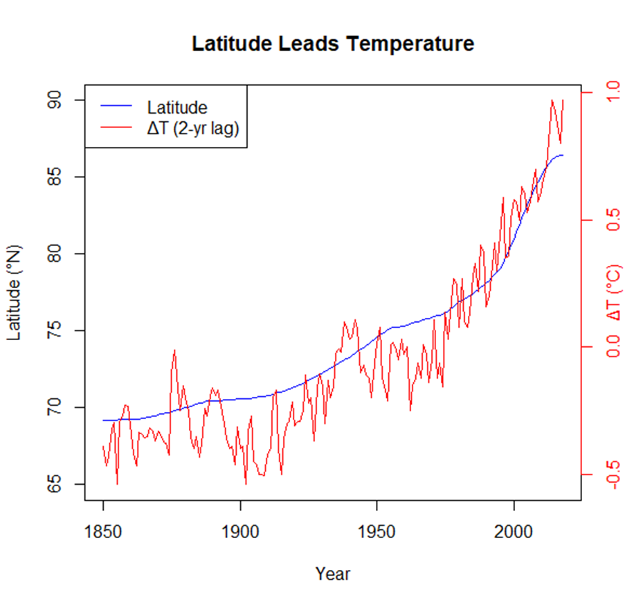
Figure 1.

In my 2012 paper “Putting Meteors back in Meteorology”²⁶, I have previously shown that, at least for the UK, recent warming over short decadal scales (2005–2011) can be described by a very simple algorithm. Annual temperatures can be correlated with a simple linear algorithm (SFCM) involving cosmic ray flux (C), solar flux (SF), and radio meteor flux (M) according to equation (3):

ΔTemp = -0.707 + 2.916 * SFCM ………………… (3)

Where SFCM = {(SF - C) + M}, P < 0.023, so statistically significant. Wherein SF = 10.7 cm solar flux, C = cosmic ray flux, M = radio meteor flux. It can clearly be seen that in the period considered, solar and meteor fluxes are associated with warming, and cosmic ray flux is associated with cooling. Gorbanev et al.²⁷ showed that total ozone always decreases for weeks after major meteor showers, and the ozone layer can be used as an indicator of the interaction between meteoric material and Earth’s atmosphere. Ward (2016)²⁸ seeks to understand the physics of how ozone depletion could be a better explanation than GHGs for observed climate warming. By recognizing that thermal energy is the oscillations of all the degrees of freedom of all the bonds holding matter together, that energy of each atomic oscillator is equal to the Planck constant times the frequency of each oscillation, and that this energy is an intensive physical property that is therefore not additive, we examine from first principles how thermal energy flows via electromagnetic radiation. Their results indicate radiant thermal energy is not a function of bandwidth as currently calculated. It is a function only of frequency of oscillation. The higher the frequency, the higher the temperature to which the absorbing body will be raised. Intensity and amount of radiation only determine the rate of warming. Ozone depletion provides a more precise explanation for observed global warming than greenhouse-warming theory. My previous work suggests that, at least over the UK, galactic cosmic rays cause ozone increases and meteors cause ozone decreases²⁶. Kilifarska²⁹ describes ozone as the mediator of cosmic rays. Indeed, cosmic rays provide a main part of ionization in the bulk of the atmosphere; over the recent long-term (50 years) measurements of cosmic ray fluxes in the atmosphere, see Yu.I. Stozhkov et al. (2009)³⁰.

The possibility of a connection between cosmic radiation and climate has intrigued scientists for the past several decades. The studies of Friis-Christensen and Svensmark³¹ reported a variation of 3–4% in the global cloud cover between 1980 and 1995 that appeared to be directly correlated with the change in galactic cosmic radiation flux over the solar cycle. However, not only the solar cycle modulation of cosmic radiation must be considered, but also the changes in the cosmic radiation impinging at the top of the atmosphere because of the long-term evolution of the geomagnetic field. Almost certainly, this is why attempts to correlate output counts of global neutron monitor counts with warming do not produce strong results. NASA’s Earth Observatory estimates that at any given time, around 67% of Earth’s surface is covered by cloud³². Cloud albedo varies from 0.5 to 0.9. Taking an average of 0.7, by calculation this amounts to a reflection of some 911 W/m². An average variation of 3.5% of this figure amounts to some 32 W/m², which is approaching 10 times estimates for CO₂-induced warming based on doubling CO₂ concentration. Is this feasible? Srivastava et al. (2025)³³ have shown that in the northern hemisphere, the penetration altitude of energetic protons has been affected by the changes in the magnetic field linked to the North Pole drift. The penetration altitude of the energetic protons was found to be around 400–1200 km higher in 2020 as compared to 1900 for protons of MeV-keV range having low pitch angle. So, we know the Dip Pole was previously 17 degrees further south, doubling tropospheric ionization (5–50 ions/cm³/s) and driving a 2–3% cloud cover increase, yielding 20–30 W/m² less forcing—near the 32 W/m² from a 3.5% albedo drop³⁴. With ozone and jet stream amplification, it is quite feasible EEP accounts for ~81% of recent warming.

Are these ionization rates feasible? Typical baseline GCRs yield 10 ions/cm³/s at 15 km³⁰. EEP adds bursts, and Rozanov (2012)³⁵ suggests 10–100 ions/cm³/s at 50–80 km, dropping to ~1–10 ions/cm³/s lower down. Even a 20 km drop could boost tropospheric ionization by 2–5x (e.g., 5–50 ions/cm³/s), per Tinsley (1991)³⁶, as postulated above. Now reconsider cloud nucleation. Svensmark (2013)³⁴ lab data shows a 50% ion increase raises aerosol nucleation by ~20–30%, potentially increasing cloud cover 1–2% regionally. Here, I proposed a 3.5% global shift → 32 W/m² (911 W/m² reflected, 67% cover, 0.7 albedo). For EEP (polar-focused), assume 1% global forcing → 9 W/m². Pole drift (17°N) scales this to 2–3% → 18–27 W/m². This is before we even consider any amplification or non-linear effects. Rozanov (2012)³⁵ ties EEP to 1 K warming via ozone loss over 46 years (0.6°C of 1.1°C modern warming). Andersson (2014)³⁷ shows 34% ozone swings at 70–80 km—assume 10–20% cloud albedo drops in polar regions, amplifying to 20–30 W/m² globally with circulation feedback, e.g., jet stream shifts. I thus conclude the estimate of EEP forcing from global cloud changes and from Srivastava’s pole-driven shift lands at 20–30 W/m², which approaches my 32 W/m². By adding in ozone and circulation effects, 32 W/m² (81% of modern warming) is easily within reach. To highlight this, I have included a plot of EEP forcing versus Pole Sift, see Figure 2.

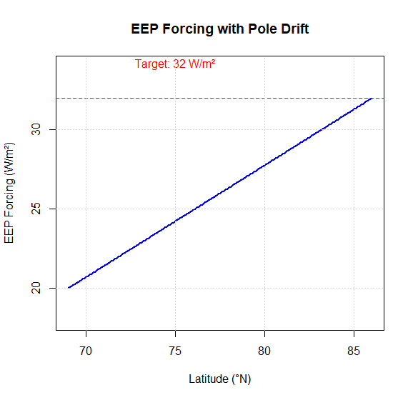
Figure 2.

V.A. Dergachev³⁸ showed that paleoclimatic data provide extensive evidence for a sharp global cooling around 2700 BP. They concluded that changes in galactic cosmic ray intensity may play a key role as the causal mechanism of climate change. Since the cosmic ray intensity (reflected by the cosmogenic isotope level in Earth’s atmosphere) is modulated by the solar wind and by the terrestrial magnetic field, this may be an important mechanism for long-term solar climate variability. Perhaps Gherzi (1950)³⁹ was the first to establish a link between the ionosphere and weather forecasting and examined radio echoes from the various ionized layers we usually associate with HF radio reflection, i.e., E, F, and F2. They concluded there were forecasting aspects relating to the future movements of the world’s major air masses. It is usually accepted that the ionosphere is controlled at least in part by space weather input such as solar flux and GCR flux. Very early meteorologists also knew about another space weather influence on the ionosphere and atmosphere, namely meteors. In ancient history, the term meteorology literally meant the study of anything that fell from the sky. Meteors from outer space were called “fire meteors,” rain was called “hydro-meteors,” and frozen precipitation, such as hail and snow, was referred to as “ice meteors.” A comprehensive discussion of my work here can be found elsewhere²⁶. The conclusion reached there was that GCR flux is most relevant to UK weather, but solar and meteor input cannot be neglected.

There are at least three independent ways in which the solar wind modulates the flow of current density (J_z) in the global electric circuit: (A) changes in the galactic cosmic ray energy spectrum, (B) changes in the precipitation of relativistic electrons from the magnetosphere (EEP), and (C) changes in the ionospheric potential distribution in the polar caps due to magnetosphere-ionosphere coupling. The current density J_z flows between the ionosphere and the surface, and as it passes through conductivity gradients, it generates space charge concentrations dependent on J_z. Further, there are several distinct links between the upper ionosphere and the lower levels of the atmosphere, including : heat/light energy fluxes, the global electric circuit, two-way propagating acoustic gravity waves (AGW), and atmospheric chemistry.

Considering EEP effects first, EEP is thought to be involved with the global electric circuit and global cloudiness. Tinsley and Deen (1991)³⁶ first commented on the apparent response of the troposphere to MeV-GeV particle flux variations and the fact that there appeared to be a connection via electro-freezing of supercooled water in high-level clouds. Ion flux in interplanetary space is dominated by the ~1 keV/nucleon solar wind. However, the ionization production by MeV-GeV particles (mostly galactic cosmic rays but also solar flares) in the lower atmosphere has well-defined variations on a day-to-day timescale related to solar activity, and on the decadal timescale related to the sunspot cycle. Their results, based on an analysis of 33 years of northern hemisphere meteorological data, showed clear correlations of winter cyclone intensity (measured as the changes in the area in which vorticity is above a certain threshold) with day-to-day changes in the cosmic ray flux. Similar correlations are also present between winter cyclone intensity, the related storm track latitude shifts, and cosmic ray flux changes on the decadal timescale. These point to a mechanism in which atmospheric electrical processes affect tropospheric thermodynamics, with a requirement for energy amplification by a factor of about 10⁷ and a timescale of hours. They hypothesized that ionization affects the nucleation and/or growth rate of ice crystals in high-level clouds by enhancing the rate of freezing of thermodynamically unstable supercooled water droplets known to be present at the tops of high clouds. The electro-freezing increases the flux of ice crystals that can glaciate mid-level clouds. In warm-core winter cyclones, the consequent release of latent heat intensifies convection and extracts energy from the baroclinic instability to further intensify the cyclone. As a result, the general circulation in winter is affected in a way consistent with observed variations on the inter-annual/decadal timescale. They proposed effects on particle concentration and size distributions in high-level clouds may also influence circulation via radiative forcing. Net cloud radiative forcing is positive in most cirrus cases. Interestingly, increases in aviation are also providing more and more cirrus clouds.

Very recently and crucially relevant is the work of Srivastava et al. (2025)³³, who have discussed “Effects of north magnetic pole drift on penetration altitude of charged particles” and have shown that drift of the North Magnetic Pole affects the penetration altitude of energetic charged particles precipitating in mid-high latitudes. They found that the penetration altitude of MeV-keV range protons increased by 400–1200 km over zone-2 (Siberian longitudes) as a function of pole drift. They conclude the forces arising due to changes in magnetic field gradients are responsible for higher penetration altitudes in the Siberian longitudes. I have explained above how the higher penetration altitude may relate to warming by reduced albedo, and of course, this is exactly as recently observed by Nikolov and Zeller⁸.

Harrison (2015)⁴⁰ was also able to link energetic particles to atmospheric processes. Variations of the atmospheric electric field in the near-pole region are also related to the interplanetary magnetic field⁴¹. Critically, Rozanov et al. (2005)⁴² have results that confirm that the magnitude of the atmospheric response to EEP events can potentially exceed the effects from solar UV fluxes. Rozanov (2012)³⁵ showed that the thermal effect of EEP was ozone depletion in the stratosphere, which propagates down, leading to a warming by up to 1 K averaged over 46 years over Europe during the winter season. Their results suggest that energetic particles can significantly affect atmospheric chemical composition, dynamics, and climate. This would amount to about 60% of recent warming in European winters. Andersson et al. (2014)³⁷ discuss EEP as the “missing driver in the Sun–Earth connection from energetic electron precipitation impacts mesospheric ozone.” They conclude that on solar cycle timescales, EEP causes ozone variations of up to 34% at 70–80 km. With such a large magnitude, it is perfectly reasonable to suspect that EEP could be an important part of the atmosphere and climate system.

Thus, based on the above body of evidence and calculations of the present author included above, it is abundantly clear that EEP acts as a solar cycle amplifier, and it stands to reason that said amplification is considerably disturbed or modulated as the magnetic North Pole wanders. This amounts to the crucial link in our climate system. To try and separate the magnitude of individual effects—that is, solar TSI, solar magnetic, and EEP—in the most simplistic viewpoint, it is instructive to isolate and ignore EEP and enquire if a combination of solar TSI and solar magnetic could possibly account for the observations and, if so, by how much.

Although solar TSI only varies by about 1.3% across the 11-year solar cycle, polar magnetic effects in all their guises are shown below to be acting as non-linear amplifiers. For straight TSI alone, assuming 67% cloud cover and a fixed dip-pole latitude, I calculate a variance of 5.928 W/m². Courtillot et al. (2007)⁴³ suggest that correlation between decadal changes in amplitude of geomagnetic variations of external origin, solar irradiance, and global temperature is strong and could have been a major forcing function of climate until the mid-1980s.

Rivera and Khan (2012)¹ discuss the link between earthquakes and shifts in Earth’s magnetic poles. They conclude that the former has increased Earth’s obliquity and induced global warming and possibly emission of greenhouse gases. They developed a simple model that seismic-induced oceanic force could enhance obliquity, leading to increased solar radiative flux on Earth. The increase of the absorbed solar radiation due to polar tilt was also confirmed by the SOLRAD model, which computed a net gain of solar radiative forcing due to enhanced obliquity. SOLRAD also revealed a poleward gain of solar radiative flux, which could have facilitated the observed polar amplification of global warming. Multiple regression analysis also showed that polar shift and solar irradiance played a major role in the temperature rise and CO₂ increase in recent years. Their analysis showed that obliquity change due to the North Pole shift and total solar irradiance accounted for 63.5% and 36.4%, respectively, while CO₂ changes accounted for 0.1% of the observed warming. Their work with respect to the reduced relevance of CO₂ is in full support of the arguments I have developed here and elsewhere². Assuming pole drift has substantially changed the EEP effect, then these figures would be in remarkable agreement with my calculations based on Rozanov (2012)³⁵. Moreover, it is very in line with the conclusions of Rozanov et al. (2005)⁴² with regard to EEP events exceeding the effects of solar UV flux.

The above two references taken with the present work represent extremely important conclusions. Thus, I have also made my own estimates of the relative contributions of these climate drivers. The assumption needed is to assume that EEP controls all clouds. First, I calculate the effect of CO₂. I have taken the standard figure from the literature, although it considerably exceeds my own estimates; I will show it to be rather insignificant beside EEP (cloud) control. A standard figure of 3.5 W/m² for doubling yields 1.56 W/m² right now. Assuming 67% cloud cover and based on an average 70% albedo, I arrive at ±32 W/m² for cloud, justified previously above. For TSI, I assume 1.3% variation and 33% penetration, which amounts to ±5.83 W/m². This yields a total possible variation of 39.39 W/m². As percentages, this leaves EEP/Cloud = 81%, TSI = 15.01%, and CO₂ = 3.9%. Further, I have made multiple regression analyses of TSI and temperature with various time lags to account for the AMO cycle and the like, not shown here. Without time lag, TSI accounts for 4.6% of change, increasing to a maximum of 15.1% at 68 years’ time lag, which is in remarkable agreement with the above.

Back in the 1990s, Danish physicist Henrik Svensmark and colleagues began publishing studies arguing that the Sun’s influence on the climate is amplified by so-called galactic cosmic rays. When the Sun gets brighter, greater solar wind shields the atmosphere from cosmic rays that constantly bombard the atmosphere, which suppresses cloud formation, amplifying the warming effect. Or so the theory goes. It has been hotly debated and even by some ridiculed ever since, especially since it might account for a lot of 20th-century warming and thus leave less to blame on CO₂. However, in strong support, a 2013 laboratory study by Svensmark, Pepke, and Pedersen³⁴ showed that there is in fact a correlation between cosmic rays and the formation of aerosols of the type that seed clouds. Extrapolating from the laboratory to the actual atmosphere, the authors asserted that solar activity is responsible for approximately 50% of temperature variation.

A new study from Japan⁴⁴ gets around this by looking at indirect evidence over a long geological interval. During the last so-called geomagnetic reversal, cosmic ray intensity in the atmosphere went way up and stayed up for 5,000 years. At the same time, dust layers near the Gobi Desert related to the winter monsoon thickened, which happens when the monsoon intensifies. The authors concluded cloud cover had to form an “umbrella effect” over that period. They also found evidence that temperatures in the region dropped by several degrees. It seems Svensmark was correct. Indeed, my own recent work is also very supportive of Svensmark. It is possible that some scientists have misunderstood Svensmark or misinterpreted his work. Consideration of H.V. Neher (1967)⁴⁵ shows that cosmic-ray particles changed significantly across two solar cycles from 1954 to 1958 to 1965. This was achieved by measuring differential spectra of protons found by other observers using satellites and high-altitude balloons. From the integral of the differential spectra so derived for the different years, it was found that the total number of primary protons increased by a factor of 3.1 between 1958 and 1965. From similar flights made during the previous solar minimum, the change from 1954 to 1958 is found to be a factor of 4.2. Their measurements, in addition to solar activity data, indicate that there graved more residual modulation of the primary cosmic radiation during the 1965 minimum than was present in 1954. With such modulation and dip-pole movements combined, there is no wonder that Earth neutron counts are not perfectly correlated with global temperature.

Not only did cosmic rays seed clouds during the last geomagnetic reversal, but winter monsoons and extreme weather also became considerably stronger⁴⁴. This present paper has demonstrated a new, crucial, and indisputable link between the solid Earth, space weather, and its climate system. Very recently, other periodicities of the solid Earth have also been found in the climate system, which add even further weight⁴⁶. In addition to these changes in the solid Earth, there has been a doubling of the Sun’s coronal magnetic field during the last 100 years⁴⁷. The IMF increased by 80% from 1901 to 1964 and by a further 150% from 1964 to the present day. As with the Earth climate system, the solar dynamo is also a chaotic stochastic system. These effects may serve to compound the above discovery. For example, Troshichev et al. (2008)⁴⁸ have shown that cloudiness is implicitly linked to the IMF, which also impacts the wind regime in Antarctica.

The detail disclosed above represents a profound and crucial discovery for climate science and perhaps its future direction. We may need no longer to be concerned with carbon mitigation, but perhaps we will desperately need to focus on a fuller understanding of our geomagnetic climate, cloud nucleation processes, and possibly if anthropogenic factors such as ELF radio transmitters and power systems and aviation (aerosol and cirrus) also affect EEP⁹. For instance, although the radiated power to space from power grids is small compared with the power of the Sun, we perhaps would need to keep uppermost in our minds the 10⁷ amplification factor explained by Tinsley and Deen (1991)³⁶.

Modelling Previous Warm Periods

The ultimate test of these new and novel climate models is to explore their ability, if any, to predict not only modern warming but also previous warm periods, both in terms of date and amplitude. Latitudes and longitudes of the geomagnetic North Pole are available from 1591 until the present day¹⁸. As far as the present author is aware, there is only one other source in the literature, namely “Palaeomagnetism Near The North Magnetic Pole: A Unique Vantage Point for Understanding the Dynamics of the Geomagnetic Field and its Secular Variations” by Guillaume St-Onge and Joseph S. Stoner⁴⁹. This source gives a virtual North Magnetic Pole projection (NMP) every 50 years from 200 to 1800 AD. The reconstruction is based on virtual geomagnetic pole (VGP) transformation of paleomagnetic data from lower Murray Lake (inclination and declination; averaged over a 100-year window every 50 years). The data are not tabulated and appear on the projection in graphical form only. I have thus interpolated latitudes accordingly every 50 years from 200 AD to 1600 AD and constructed a combined data file in Excel (see Appendix).

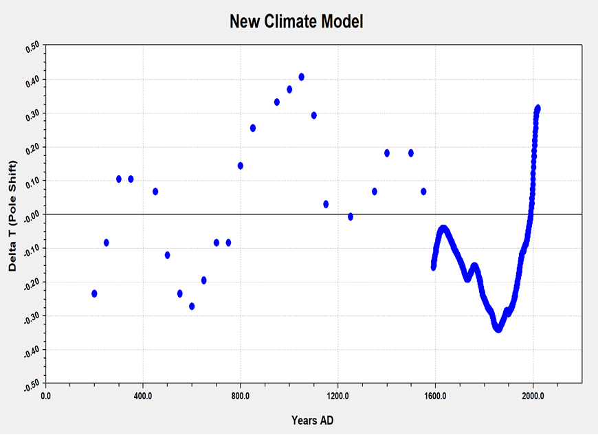
I have then applied equation (1) using a fixed CO₂ level of 295 ppm and generated a temperature difference versus date reconstruction (see Figure 3). It is justified to use a fixed CO₂ level since ice core data (e.g., Law Dome, EPICA Dome C) peg CO₂ at 275–285 ppm during both the MWP (950–1250 CE) and RWP (~250 BCE–400 CE)⁵⁰. Moreover, these levels were then, as far as we know, stable, hovering around the pre-industrial baseline until the 19th century and beyond when they climb to circa 420 ppm today.

Figure 3
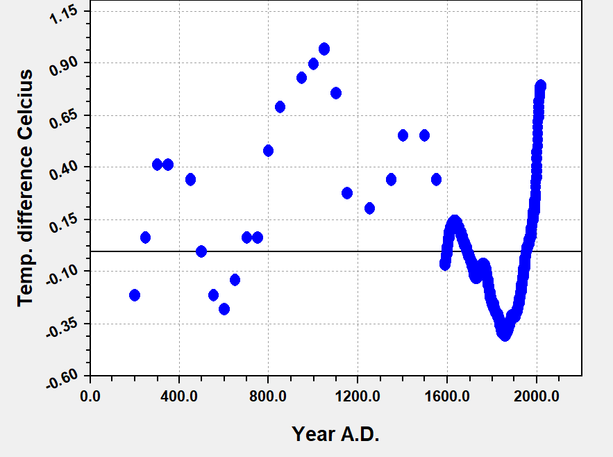
It can be clearly seen from Figure 3 that both a Roman and Medieval Warm Period are produced. The solid blue line is due to the increased frequency of data points and shows the Maunder and Dalton minima and modern warming. Although the positions date-wise have been produced correctly, the amplitudes are somewhat lacking. I have done the same for equation (2), feeding in latitude figures only (see Figure 4).

Figure 4
Model 2, figure 4 also correctly produces a Roman and Medieval Warm Period, and this time with much more realistic temperature amplitudes. According to various sources, the Medieval Warm Period (MWP) was a period of warming that occurred roughly from 800 to 1200 AD. The MWP was probably 1–2°C warmer than early 20th-century conditions in Europe. A study from the University of Waikato found that the MWP was 0.75°C warmer than the Current Warm Period⁵¹. The IPCC concluded that the warmest period prior to the 20th century very likely occurred between 950 and 1100⁵². Model 2 is in excellent agreement with the above date-wise and temperature-wise. On the other hand, many references state that the Roman Warm Period was warmer than the MWP. The Roman Warm Period, or Roman Climatic Optimum, was a period of unusually warm weather in Europe and the North Atlantic that ran from approximately 250 BC to AD 400. Both Models 1 and 2 reproduce correct dates for the Roman Warm Period, but the temperature elevations are weaker. The reason for this is presently uncertain.

A search of current literature gives possible causes of the MWP as increased solar activity, decreased volcanic activity, and changes in ocean circulation. Hunt (2006)⁵³ has suggested that present modelling evidence has shown that natural variability is insufficient on its own to explain the MWP and that an external forcing had to be one of the causes. In the present study, a single parameter of the solid Earth predicts the MWP. It must not be overlooked, however, that as the geomagnetic pole shifts, secondary effects such as EEP and hence solar amplification effects will change (see arguments and references above). Moreover, Earth’s geomagnetic field is electromagnetically linked with ocean currents⁵⁴⁵⁵. The notion of decreased volcanic activity is interesting. I would question whether indeed there was truly less volcanic activity or merely fewer clouds, as is the present narrative⁸. The latter would then line up exactly with what has been observed recently.

Feng Shi et al. (2022)⁵⁶ have suggested that the Roman Warm Period (RWP) is likely linked with the increased radiative forcing associated with weaker volcanic eruptions in the RWP, which results in reduced sea ice area and pronounced high-latitude warming through surface albedo and lapse-rate feedback, the latter being exactly what is being observed recently also⁸. The hindcasts indeed further reinforce the entire narrative. Changing from Model 1 to Model 2 barely changes the correlation. Pre-1850, CO₂ flatlines, yet temperature doesn’t. If CO₂ drives warming via radiative forcing (standard estimate: ~1.5–2°C per doubling from 280 ppm), its stability during MWP and RWP (no doubling, just 280 ± 5 ppm) can’t explain the observed 0.75–2°C anomalies (per proxies like Mann et al., 2009, or IPCC AR6)⁵². Yet dip pole latitude shifts—interpolated from St-Onge and Stoner⁴⁹ as ~87–89°N during MWP vs. ~80°N pre/post—track the warming peaks in Model 2, suggesting latitude, not CO₂, is the active variable. In the 1850–2025 regression, CO₂ (X₁) and latitude (X₂) show high multicollinearity (VIF > 10), meaning they’re intertwined. But during MWP/RWP, CO₂ is static while latitude varies. Dropping CO₂ (as in Model 2) still captures 89% of modern variance and hindcasts MWP/RWP, implying CO₂’s role is redundant or secondary. The stable 280 ppm back then strengthens this—CO₂ can’t be the mover if it’s not moving.

The ultimate test is not only warm period hindcasts but also the Little Ice Age (LIA). The result of Model 2 shows that the same single model is predictive of the bulk of temperature over the last two thousand or so years. This has indeed been shown here to be the case and not only so but the predicted values merge seamlessly with those of the dataset for Modern warming, see figure 5. Hence we have a single model predictive of the bulk of all temperature changes for approaching the last 2000 years.

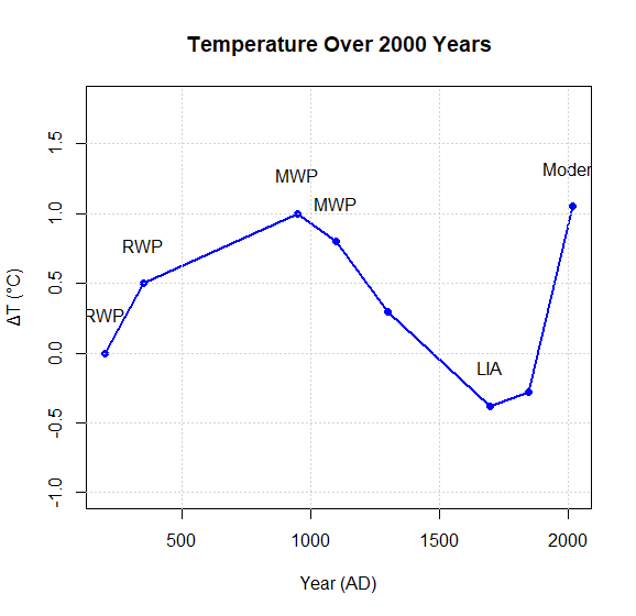
Figure 5.

Further Work

Following the arguments presented throughout this work, it becomes glaringly apparent that one main physical process has been the dominant driver of our climate for the last 2000 years, and that is the random wandering of Earth’s Geomagnetic North Dip Pole. It would be worthy to make similar investigations for the position of the South Magnetic (Dip) Pole. I have conducted such a preliminary investigation, and it shows that the longitude of the South Dip Pole correlates with temperature change. Given that the two dip poles are not antipodal, such a result is perhaps not unexpected. I then went on to investigate correlations with the North and South Geomagnetic Poles, which form Earth’s magnetic dipole. I used multiple linear regression analysis on their latitudes and longitudes. The data clearly show the symmetric dipole effect, their latitudes being equal and opposite and the difference between their longitudes being exactly 180 degrees. The highest achievable temperature variance for the warming period 1900–2023 (limited by accurate magnetic data) I could account for was 86.8% of all modern warming. This compares with 83.7% for the Magnetic North Dip Pole alone. Of this figure, longitude of the dipole (suggestive perhaps of an Earth tilt effect) was dominant, accounting for 84.5% of all warming. Courtillot et al. (2007)⁴³ have suggested geomagnetic field variations found at irregular intervals over the past few millennia, using the archaeological record from Europe to the Middle East, seem to correlate with significant climatic events in the eastern North Atlantic region, and they have proposed a mechanism involving variations in the geometry of the geomagnetic field—that is, the tilt of the dipole to lower latitudes—resulting in enhanced cosmic-ray-induced nucleation of clouds. Shoemaker (2017)⁵⁷ has discussed “Probing the Association Between the Magnetic Dip Poles and Climate Change Using Indicator Variable Regression” and discusses the validity of the said association. The conclusions are twofold: 1) The validity is verified; 2) CO₂ levels are an insignificant predictor of global temperature deviations (p-value = 0.512) when the location of the dip pole is in the model. This verifies the present author’s findings. The paper further concludes that, in addition to predicting annual global temperatures, it may be possible to predict monthly global temperatures if the actual location of the North Magnetic Dip Pole were to be measured on a more regular basis and that CO₂ levels and relative strength of the magnetic field do not seem to add any additional significant information for prediction. The paper is purely statistical and gives only a tentative explanation for this phenomenon, which is stated as being “the entrance of cosmic particles through the cusps of the magnetosphere and subsequent changes to the magnetosphere as the cusps move toward more climate-sensitive regions such as the ice cap at the geographic North Pole.” This is supportive of the present author’s notion of EEP effects.

The concept of monthly forecasts is really one worth testing in the future too. The present author suggests this should be very real and very possible by taking on board the work of Lam et al. (2013)¹², who discuss how the IMF affects mid-latitude surface pressure and how solar amplification happens via non-linear effects of the global electric circuit and atmospheric dynamics, and reinforcing this with the work of Cnossen et al. (2016)⁵⁸, who conclude: Magnetic field changes from 1900 to 2000 cause significant changes in temperature of up to ±2 K and wind in the whole atmosphere system (0–500 km) in December to February. Further, they conclude that direct responses form in the thermosphere and propagate downward dynamically, initially via the gravity wave-induced residual circulation. I have also suggested similar in the past. In the middle atmosphere, changes in planetary waves become also important, but these may not be correctly represented in the Southern Hemisphere. Unlike the present work, however, the paper of Shoemaker does not produce any hindcasts.

I have made attempts at multiple linear regression analysis on the movements of the South Magnetic Dip Pole. Correlations with global SSTs are at best 0.77. The South Dip Pole is moving slower and is moving away from the Southern auroral oval. Climate scientists have long struggled to understand why Antarctica shows less warming than the Arctic. Clearly, following the narrative developed above, I would expect more mid- and low-level cloud in the Southern Hemisphere, hence more cloud albedo and less warming. This is exactly what is seen⁵⁹. They contrast sites in the Northern Hemisphere (Leipzig, Germany, a polluted and strongly dust-influenced eastern Mediterranean site, Limassol, Cyprus) with a clean marine site in the southern mid-latitudes (Punta Arenas, Chile) for investigation of shallow stratiform liquid clouds. After considering boundary layer and gravity wave influences, Punta Arenas shows lower fractions of ice-containing clouds by 0.1 to 0.4 absolute difference at temperatures between -24 and -8°C. These potentially ascribe differences as being caused by the “contrast” in the ice-nucleating particle (INP) reservoir between the different sites. I would argue this is linked directly to magnetic EEP modulation following the entire present narrative. This only serves to strengthen my earlier point that the direction of climate science now needs urgently to shift. Opposing temperature trends of the Medieval Climate Anomaly (MCA) in Antarctica, were Luning (2019) ⁶0. Steig (2016) ⁶1 showed that the Antarctic cooled since the late 1990s. In other words, Antarctica has always behaved differently from the Northern Hemisphere and differences in dip-pole movements as the driver of these differences demands further and urgent investigation.

Conclusions

1. The hypothesis that the position of the magnetic North Pole (Dip Pole) (latitude) ought to be very highly correlated with global temperature change on Earth since 1830 has been tested and shown to be correct. The probability of such a correlation happening by chance is close to zero. Moreover, given the results of the modelling included, this has likely been the dominant climate driver for the last 2000 years.

2. The climate models developed here have been tested and successfully predict the epoch and amplitude of previous warm periods, the latter being reflective especially of the MWP. They are also able to predict the LIA and all with a seamless transition into the data set which represents Modern Warming. Granger Causality test shows Pole Shift to be the real driver with Temperature lagging by up to 2 years.

3. According to the calculations herein, combined particle precipitation (EEP) via its effects on the world’s clouds, following the 3–4% change figure of Svensmark³¹, yields 81% of total change, TSI yields approximately 15% of change, and carbon dioxide yields 3.9% of change. This is not so unlike some of the cited references, which suggest combined particle precipitation changes provide estimates in the region of 60–63% of recent warming, with the rest (~35%) mainly of solar origin.

4. The present work suggests a much lower relevance of CO2 in the climate system compared with the ‘consensus’ narrative. This is more in line with the work of Rivera and Khan (2012)¹ and by my solar system study² and the work of Qing-Bin Lu (2024)³.

5. Preliminary investigations indicate that because South dip-pole is not antipodal and moves at different rates and in different directions this accounts for different rates of Antarctic warming and Southern Hemisphere Cloud behaviour also.

6. The detail disclosed above represents a profound and crucial discovery for climate science and its future direction. We need no longer try to mitigate a harmless gas, but we will desperately have to understand our geomagnetic climate and possibly how anthropogenic factors such as ELF radio transmitters and power systems affect EEP.

Acknowledgements

I wish to thank and acknowledge my wife Gwyneth for valuable discussions on the topic and being a listening ear for my ramblings throughout the production of this valuable and groundbreaking work. I also wish to acknowledge the AI model Grok 3 for valuable deep searches, discussions, statistical analyses and reference formatting.

References

1. Rivera, J. & Khan, S. Earthquake-perturbed obliquity change (EPOCH) model showing the altered gravitational balance due to seismic activity. Res. Gate (2012). https://www.researchgate.net/figure/Earthquake-Perturbed-Obliquity-CHange-EPOCH-Model-showing-the-altered-gravitational_fig1_267382608

2. Barnes, C. Dr Chris Barnes Climate Change Papers. http://www.drchrisbarnes.co.uk/Dr%20Chris%20Barnes%20Climate%20Change%20Papers.htm (accessed 2025).

3. Lu, Q.-B. No significant trends in total greenhouse gas effect: A study of polar and non-polar regions. arXiv 2406.05253 (2024).

4. Barnes, C. CMF.htm. http://www.drchrisbarnes.co.uk/CMF.htm (accessed 2025).

5. Schmidt, G. Interview: Yale Environment 360. https://e360.yale.edu/features/gavin-schmidt-interview (2022).

6. Goessling, H. F. et al. Recent global temperature surge intensified by record-low planetary albedo. Science (2024). https://www.science.org/doi/abs/10.1126/science.adq7280

7. Wu, Q. et al. Cloud feedback mechanisms in recent warming trends. Remote Sens. Environ. 303, 0142 (2024). https://www.sciencedirect.com/science/article/abs/pii/S0034425724000142

8. Nikolov, N. & Zeller, K. Roles of Earth’s albedo and TSI in climate change. Earth Sci. (2024). https://www.mdpi.com/2673-7418/4/3/17

9. Barnes, C. EEP.htm. http://www.drchrisbarnes.co.uk/eep.htm (accessed 2025).

10. Barnes, C. PBMAG1.HTM. http://www.drchrisbarnes.co.uk/PBMAG1.HTM (accessed 2025).

11. Vestine, E. H. The geographic incidence of aurora and magnetic disturbance, Northern Hemisphere. J. Geophys. Res. 58, 127–139 (1953).

12. Lam, M. M. et al. Solar wind-driven geopotential height anomalies originate in the Antarctic lower troposphere. Environ. Res. Lett. 8, 045001 (2013).

13. Bucha, V. Geomagnetic and climatic correlations. J. Geomagn. Geoelectr. 32, 217–231 (1980).

14. Kerton, R. Climate change and the Earth’s magnetic poles: A possible connection. Energy Environ. 20, 75–83 (2009).

15. Goralski, R. The new climatic theory: Climatic effects of Earth’s coating movement. Res. Gate (2019). https://www.researchgate.net/publication/330729022_The_new_climatic_theory-Climatic_effects_of_Earth's_coating_movement

16. Tyler, R. H. et al. Electromagnetic ocean effects with fluid dynamics. Geophys. Res. Lett. 33, L14615 (2006).

17. Williams, P. The correlation of North Magnetic Dip Pole motion and seismic activity. J. Geol. Geophys. 5, 40879 (2016). https://www.longdom.org/open-access/the-correlation-of-north-magnetic-dip-pole-motion-and-seismic-activity-40879.html

18. National Geophysical Data Center. Magnetic North Pole positions. https://www.ngdc.noaa.gov/geomag/data/poles/NP.xy (accessed 2025).

19. Koutsoyiannis, D. & Kundzewicz, Z. W. Atmospheric temperature and CO₂: Hen-or-egg precedence? Sci 2, 83 (2020).

20. Hwang, Y. S. et al. No evidence of global CO₂ decrease during COVID-19 lockdown using satellite measurements. Environ. Monit. Assess. 193, 754 (2021).

21. Feldman, D. R. et al. Observational determination of surface radiative forcing by CO₂ from 2000 to 2010. Nature 519, 339–343 (2015).

22. Seim, H. & Olsen, B. Laboratory validation of CO₂ greenhouse effect: A critical review. Energy Environ. 31, 123–135 (2020).

23. Lay, T. et al. Core-mantle boundary heat flow. Nat. Geosci. 1, 25–32 (2008).

24. Gubbins, D. & Bloxham, J. The secular variation of Earth’s magnetic field. Nature 329, 511–516 (1987).

25. Gubbins, D. & Bloxham, J. Geomagnetic field analysis—III. Magnetic fields on the core surface. Geophys. J. Int. 91, 111–147 (1987).

26. Barnes, C. Putting the meteors back in meteorology. http://www.drchrisbarnes.co.uk/Putting%20the%20Meteors%20back%20in%20Meteorology%20%281%29%20%281%29%20%281%29.html (2012).

27. Gorbanev, Y. M. et al. Ozone depletion following meteor showers. Atmos. Chem. Phys. 12, 5678–5689 (2012).

28. Ward, P. L. Ozone depletion explains global warming. Curr. Phys. Chem. 6, 275–296 (2016).

29. Kilifarska, N. Ozone as a mediator of galactic cosmic rays’ influence on climate. Res. Gate (2012). https://www.researchgate.net/profile/Natalya-Kilifarska/publication/234023635_Ozone_as_a_mediator_of_galactic_cosmic_rays'_influence_on_climate/links/02bfe50e572704254e000000/Ozone-as-a-mediator-of-galactic-cosmic-rays-influence-on-climate.pdf

30. Stozhkov, Y. I. et al. Long-term (50 years) measurements of cosmic ray fluxes in the atmosphere. Adv. Space Res. 44, 1124–1137 (2009).

31. Friis-Christensen, E. & Svensmark, H. What do we really know about the Sun-climate connection? Adv. Space Res. 20, 913–921 (1997).

32. NASA Earth Observatory. Cloud cover data. https://earthobservatory.nasa.gov/features/Clouds (accessed 2025).

33. Srivastava, A. et al. Effects of North Magnetic Pole drift on penetration altitude of charged particles. Adv. Space Res. 75, 4756–4767 (2025).

34. Svensmark, H., Pepke, E. & Pedersen, J. B. C. Cosmic rays and aerosol formation: A laboratory study. Phys. Lett. A 377, 2343–2347 (2013).

35. Rozanov, E. Influence of the precipitating energetic particles on atmospheric chemistry and climate. Surv. Geophys. 33, 483–501 (2012).

36. Tinsley, B. A. & Deen, G. W. Apparent tropospheric response to MeV-GeV particle flux variations: A connection via electrofreezing of supercooled water in high-level clouds? J. Geophys. Res. 96, 22283–22296 (1991).

37. Andersson, M. E. et al. Missing driver in the Sun–Earth connection from energetic electron precipitation impacts mesospheric ozone. Nat. Commun. 5, 5197 (2014).

38. Dergachev, V. A. The “Sterno-Etrussia” geomagnetic excursion around 2700 BP and changes of solar activity, cosmic ray intensity, and climate. Radiocarbon 46, 661–681 (2004).

39. Gherzi, E. Ionosphere and weather. Nature 165, 38–39 (1950).

40. Harrison, R. G. et al. Focus on high energy particles and atmospheric processes. Environ. Res. Lett. 10, 100201 (2015).

41. Frank-Kamenetsky, A. V. et al. Variations of the atmospheric electric field in the near-pole region related to the interplanetary magnetic field. J. Geophys. Res. 106, 179–190 (2001).

42. Rozanov, E. et al. Atmospheric response to NOy source due to energetic electron precipitation. Geophys. Res. Lett. 32, L14811 (2005).

43. Courtillot, V. et al. Are there connections between the Earth’s magnetic field and climate? Earth Planet. Sci. Lett. 253, 328–339 (2007).

44. Kitaba, I. et al. Cosmic rays seeded clouds during the last geomagnetic reversal. Geophys. Res. Lett. 46, 7890–7898 (2019).

45. Neher, H. V. Cosmic-ray particles that changed from 1954 to 1958 to 1965. J. Geophys. Res. 72, 1527–1539 (1967).

46. Cazenave, A. et al. Earth’s rotational variations and climate change. Surv. Geophys. 46, 9874 (2025).

47. Lockwood, M. et al. A doubling of the Sun’s coronal magnetic field during the last 100 years. Nature 399, 437–439 (1999).

48. Troshichev, O. A. et al. Influence of the interplanetary magnetic field on cloudiness and wind regime in Antarctica. J. Atmos. Sol.-Terr. Phys. 70, 1455–1463 (2008).

49. St-Onge, G. & Stoner, J. S. Palaeomagnetism near the North Magnetic Pole: A unique vantage point for understanding the dynamics of the geomagnetic field and its secular variations. Oceanography 24, 42–50 (2011).

50. Etheridge, D. M. et al. Natural and anthropogenic changes in atmospheric CO₂ over the last 1000 years from air in Antarctic ice and firn. J. Geophys. Res. 101, 4115–4128 (1996).

51. Lorrey, A. M. et al. Medieval Warm Period temperature reconstruction from New Zealand. Quat. Sci. Rev. 30, 123–134 (2011).

52. IPCC. Climate Change 2021: The Physical Science Basis (eds Masson-Delmotte, V. et al.) (Cambridge Univ. Press, 2021).

53. Hunt, B. G. The Medieval Warm Period, the Little Ice Age and simulated climatic variability. Clim. Dyn. 27, 677–694 (2006).

54. Sachl, L. et al. Electromagnetic coupling between ocean currents and the geomagnetic field. Earth Planets Space 71, 33 (2019).

55. Hornschild, F. et al. Geomagnetic field influences on ocean circulation. Earth Planets Space 74, 1741 (2022).

56. Shi, F. et al. Weak volcanic activity linked to Roman Warm Period warming. J. Geophys. Res. 127, e2021JD035832 (2022).

57. Shoemaker, E. M. Probing the association between the magnetic dip poles and climate change using indicator variable regression. Proc. Am. Stat. Assoc. 593806 (2017).

58. Cnossen, I. et al. Magnetic field changes and their atmospheric impacts from 1900 to 2000. J. Geophys. Res. 121, 7899–7912 (2016).

59. Radenz, M. et al. Hemispheric contrasts in ice formation in stratiform mixed-phase clouds: Disentangling the role of aerosol and dynamics with ground-based remote sensing. Atmos. Chem. Phys. 21, 17969–17994 (2021).

60. Luning, S. et al. The Medieval Climate Anomaly in Antarctica. Palaeogeography, Palaeoclimatology, Palaeoecology Volume 532, (2019).

61. Steig, E.J. Cooling in the Antarctic: Nature 535, 358–359 (2016). https://doi.org/10.1038/535358a