A New Method for Medium Term Temperature Anomaly Forecasting and Climate Prediction by Dr Chris Barnes, Bangor Scientific and Educational Consultants, email manager@bsec-wales.co.uk homepages http://drchrisbarnes.co.uk and http://bsec-wales.co.uk Published 22^nd May 2015, Revised June 2015.

Abstract

A New Method for Medium Term Temperature (summer season) Anomaly Forecasting and Climate Prediction is introduced based solely on a polynomial data file linked QBO and temperature behaviour in North Wales since 1948. The key is in choosing two months to establish QBO rate of change, here the preceding January and April are employed. Complex climate modelling is NOT required because the qbo via its tele-connections is a complex and multivariate indicator of drivers from above and below including natural drivers such as solar and volcanism in addition to anthropogenic drivers such as greenhouse gases, wind farms, power systems, radio transmitters and aviation. Taking a naïve approach to results leads to a perceived warming of about .22 C per decade which is consistent with the IPCC’s most recent estimates. However, taking a more detailed analysis leads to a cyclic understanding of recent warming and cooling in terms of solar and volcanic activity. The infamous ‘hockey stick’ period of warming may have been created by a coincidental combination of a fall in volcanism and a rise in solar activity the likes of which may only be seen either once every 792 years ; 2640 years or 5192 years based on combinations of the three known volcanic, seismic and Gleissberg cycles. The first two of these take us back to the medieval warm period and Roman warm period consecutively. At least in North Wales it would appear we have now entered into a cooling phase which could last several decades.

Introduction

Forecasting the weather for the long and medium range has always been considered a difficult and scientifically challenging problem. Traditional methods are based on climate models of ever increasing complexity and immense computing power. Some have argued on theoretical grounds that even if we have an almost perfect model with almost perfect initial data, we will never be able to make an accurate weather prediction more than a few weeks ahead.

The method described here employs use of the QBO, specifically the value of the 30mb equatorial zonal wind index and strives to forecast anomaly for a complete season rather than on a day by day or week by week basis.

The quasi-biennial oscillation (QBO) is a quasi-periodic oscillation of the equatorial zonal wind between easterlies and westerlies in the tropical stratosphere with a mean period of 28 to 29 months. The alternating wind regimes develop at the top of the lower stratosphere and propagate downwards at about 1 km (0.6 mi) per month until they are dissipated at the tropical tropopause. Downward motion of the easterlies is usually more irregular than that of the westerlies. The amplitude of the easterly phase is about twice as strong as that of the westerly phase. At the top of the vertical QBO domain, easterlies dominate, while at the bottom, westerlies are more likely to be found.

The QBO was discovered in the 1950s by researchers at the UK Meteorological Office (Graystone 1959) [1], but its cause remained unclear for some time. Rawinsonde soundings showed that its phase was not related to the annual cycle, as is the case for many other stratospheric circulation patterns. In the 1970s it was recognized by Richard Lindzen and James Holton [2] that the periodic wind reversal was driven by atmospheric waves emanating from the tropical troposphere that travel upwards and are dissipated in the stratosphere by radiative cooling. The precise nature of the waves responsible for this effect was then heavily debated; in recent years, however, gravity waves have come to be seen as a major contributor and the QBO is now simulated in a growing number of climate models (Takahashi 1996, Scaife et al. 2000, Giorgetta et al. 2002) [3-5].

Effects of the QBO include mixing of stratospheric ozone by the secondary circulation caused by the QBO, modification of monsoon precipitation, and an influence on stratospheric circulation in northern hemisphere winter (mediated partly by a change in the frequency of sudden stratospheric warmings). Westward phases of the QBO often coincide with more sudden stratospheric warmings, a weaker Atlantic jet stream and cold winters in Northern Europe and eastern USA whereas eastward phases of the QBO often coincide with mild winters in eastern USA and a strong Atlantic jet stream with mild, wet stormy winters in northern Europe (Ebdon 1975) [6].

Hypothesis

As stated above, it has recently been acknowledged that the QBO (quasi-biennial oscillation) might influence Atlantic storm tracks and therefore British weather. Baldwin and Dunkerton (1999) [7] showed by observation that large variations in the strength of the stratospheric circulation, appearing first above 50 kilometres, descend to the lower most stratosphere and are eventually followed by anomalous tropospheric weather regimes. Further that during the 60 days after the onset of these events, average surface pressure maps resemble closely the Arctic Oscillation pattern. These stratospheric events also precede shifts in the probability distributions of extreme values of the Arctic and North Atlantic Oscillations, the location of storm tracks, and the local likelihood of mid-latitude storms. Our observations suggest that these stratospheric harbingers may be used as a predictor of tropospheric weather regimes.

Indeed, I have recently shown a new method of prediction using QBO. However, QBO prediction methods appear to be limited at certain time of the year [8].

To me it feels as though this limitation is just a matter of data processing/extraction. It seems to me that QBO ought to be influenced from above and below in the atmosphere due to multiple coupling mechanisms and ought ultimately to hold the secrets quasi periodic behaviour of the climate system in response to the solar cycle/ gamma ray/ meteoric inputs from above and interplay with other planetary and gravity wave systems from below. Indeed in agreement with my thoughts, the Solar signal has been found in the QBO by Cordero and Nathan (2005) [9]. Unique to their model are wave-ozone feedbacks, which provide a new, nonlinear pathway for communicating solar variability effects to the QBO. Of course anthropogenic activity too modulates atmospheric ozone concentration and will also impart onto the QBO.

Dunkerton (2012) [10] has also considered the role of gravity wave momentum transport in the quasi-biennial oscillation (QBO) was also investigated using a two-dimensional numerical model. In order to obtain an oscillation with realistic vertical structure and period, vertical momentum transport in addition to that of large-scale, long-period Kelvin and Rossby-gravity waves was necessary. The total wave flux required for the QBO was found to be sensitive to the rate of upwelling, due to the Brewer-Dobson circulation, which can be estimated from the observed ascent of water vapour anomalies in the tropical lower stratosphere. Although mesoscale gravity waves contribute to mean flow acceleration, it was thought unlikely that the momentum flux in these waves is adequate for the QBO, especially if their spectrum is shifted toward westerly phase speeds.

Short-period Kelvin and inertia-gravity waves at planetary and intermediate scales also transport momentum. His numerical results suggested that the flux in all vertically propagating waves (planetary-scale equatorial modes, intermediate inertia-gravity waves, and mesoscale gravity waves), in combination, was sufficient to obtain a QBO with realistic Brewer-Dobson upwelling if the total wave flux is 2–4 times as large as that of the observed large-scale, long-period Kelvin and Rossby-gravity waves. Lateral propagation of Rossby waves from the winter hemisphere is unnecessary in this case, although it may be important in the upper and lowermost levels of the QBO and subtropics.

Campbell has also supported the gravity wave idea and discusses non- linear propagation, amplification and wave breaking [11].

Ern et al (2014) have confirmed the importance of gravity waves by satellite studies. Ern et al (2015) have further discussed the interplay of gravity waves, the QBO and the SAO [12].

Thus I feel we need not necessarily need to model every single planetary oceanic and atmospheric component in order to make predictions about climate, but merely should plot the time domain behaviour of one dominant, yet heavily modulated, system such as the QBO.

Following this logic and since there are tele-connections between the equatorial stratospheric QBO and other parts of the planet’s climate system it ought to be possible to predict a given climatic anomaly somewhere on the planet, in the case of this paper the area local to Bangor, North Wales, and the QBO rate of change of the descent rate prior in time. In order to simplify calculation simply the 30 mb QBO zonal wind index is employed and the rate of change of the descent rate is estimated from normalised differences between the QBO value in January and that in April, this latter month being some 60 days prior to the summer season concerned. Further, the beauty of this method is that it automatically takes into account anthropogenic inputs as well. Indeed, assuming all other inputs to have produced the same sorts of effects over time, which may be questionable due to the recent very steep decline in solar Ap, it may, conceivably even, be possible to use hind-cast to decouple the effects of anthropogenic warming. For instance, it is crucial for us to consider that the most significant gravity waves which drive/modulate the QBO are created by deep convection which in turn depends on global temperature and global hydrology.

Other new anthropogenic factors may also be at play. For example the world’s wind farms, the density of which has grown almost exponentially in the last 15 years or so is also an important and new source of gravity waves. I have also previously suggested that the world’s electricity grids and any or all high power radio transmitters could also be important but hitherto unsung sources of anthropogenic gravity waves [13]. I have previously also commented on the huge impact of aviation on climate and proposed these are due changed methods of flying, fuels engine technology and flight density. All also will be expected to have both direct and indirect effects on gravity waves and hence the QBO.

Data Sets

The graphic at http://www.cpc.ncep.noaa.gov/products/CDB/Tropics/figt3.gif[14] was used for QBO data from 1996 to present and reasonably accurate 30mb equatorial zonal wind data is available back as far as 1948, see http://www.esrl.noaa.gov/psd/data/correlation/qbo.data [15].

A met office data set [16] was used to estimate the maximum temperature anomaly in Bangor and the surrounding area.

Results

An XL spreadsheet (not shown here) was constructed and used for initial data processing. A data set was sought covering as many different instances of QBO difference between the months of January and April as possible. The entire QBO data set from 1948 to 2014 was employed. The resultant January to April difference values were plotted (figure 1) against temperature anomaly using Hyams curve fitting software as shown below. Clearly a multivariate response is expected in the QBO in response to the factors mentioned above. Not surprisingly then, the best fit was a fourth order polynomial equation with R circa .32. With 67 degrees of freedom this is statistically very relevant and gives a p value of .0098.

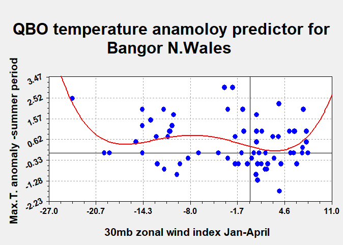
Figure 1

The best fit forecast algorithm is:

Delta T (Bangor, Wales) = 0.295 -.093 D + 0.005 D^2 + 0.0015 D^3 + 0.000054 D^4

Where D= 30mb QBO in January – 30mb QBO in April

Discussion

Maximum temperature anomaly seems to occur both when the rate of change of QBO descent ( QBO of either phase) between January and April is either maximised, however there is a tendency for a secondary somewhat weaker maximum when the value is –ve and between about a quarter and a third of its maximum negative value. There is least temperature anomaly for the period when D is positive and about a third of its maximum possible value.

Hind-cast experiments to model climate anomaly and discussion on climate change.

The forecast algorithm developed above represents best response averages for the entire period in terms of both solar and anthropogenic inputs and can be tested by making hind-casts of summer temperature anomaly on a decadal scale for period 1948 onwards. Linear regressions can then be set up to test the validity of the anomaly hind-casts against temperature anomaly calculated from real historic temperature measurements. This way it not only ought to be possible to see how good the model is but it may be possible to see how climate has changed/evolved across the 66 year period by looking at the regression constants and slopes. The regression constants ought to give a degree of information on climate warming or cooling over the period. Whereas the regression slopes ought to give a degree of information on just how much climate has been linked to QBO over the period. Finally, the regression coefficients themselves ought to give a degree of information on the reliability of the data for each decade investigated.

Thus it is instructive to consider each regression and then consider the constant (temperature intercept), the ‘x’ coefficient (slope) and the regression factor for each regression. For example, the result for the decade 1948-1958 is shown in figure 2 below:

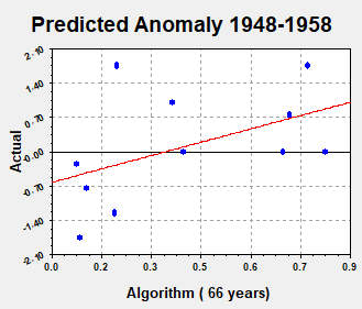TI = -.67; slope = 1.94; R =.48 p=.089

Figure 2

The results for the other decades and the final period considered, namely 2003 -2014 are shown in table 1 below:

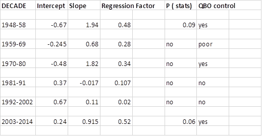
Table 1

It is instructive to note that the most statically relevant period appears to be the most recent, i.e. the period 2003-2014.

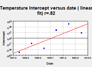
Consider figure 3, temperature intercept first. This gives a measure of the background temperature in each decade compared with the average for the whole 66 year period.

Figure 3

If a linear spline were to be applied it would be apparent that this figure was rising in the first decade considered, then falling, then rising steeply from the 70’s to the 80’s then rising less steeply in the 1990’s and in the last period considered from 2003 -2014 the figure is falling. This seems to be roughly in line with what has been reported by climate scientists elsewhere but note here this behaviour has been obtained by a totally unique and independent method. Some have suggested that the most recent cooling is only short term, see for instance but not exclusively, Grenier et al (2015) and that it may proceed up until about 2035 [17].

If a linear regression (trend line) is applied a slope of about .22 C per decade is deduced. If one were naïve in analysis, one would stop at this point and conclude that the result is highly suggestive of climate warming on the same scale as that presently predicted by IPCC. Certainly with p=.012 there is also some perceived statistical significance to the result.

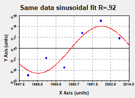
However, it is well worth considering if these data could fit another interpretation. For instance, when a sinusoidal fit is applied a far better regression factor is obtained, R =.92. The P Value Results for r=.92 DF=6 are that the two-tailed P value equals 0.0012. By conventional criteria, this difference is considered to be very statistically significant and is far more so than for the linear trend line.

In this case, a half-cycle with a length of some 40 years is observed. Double this is the familiar Gleissberg cycle of 72-88 years. The importance of solar cycles is discussed at http://www.newclimatemodel.com/the-importance-of-solar-cycles-2/. [18].

Thus based on the sinusoidal interpretation, the suggestion is that at least the summertime climate of North Wales is now very much entering into a cooling phase. Grenier et al (2015) [17] discuss cooling scenarios between 2006 and 2035. Taking the observation here that cooling probably began about 8-10 years prior leads me to the conclusion that this cooling could well be solar and part of the natural Gleissberg cycle. Delworth, Rosati et al (2015) [19] have discussed a link between the hiatus in global warming and the recent North American droughts including pacific/ northern hemisphere teleconnections.

To elucidate this behaviour, it is further instructive to consider the temporal behaviour of the ‘x’ coefficient from the regressions. This has been done in figure 4 below. The larger its value the more strongly the QBO influences climate. R=.9.

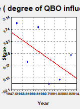
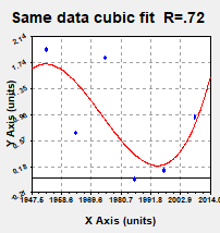
Figure 4 (a) trend line (b) cubic fit (c) sinusoidal fit

Taking a naïve approach would be simply to look at the trend line which has a negative slope but a relatively weak regressions factor hence of little or no statistical significance but yet which would suggest a weakening of QBO (e.g. pacific) influence. This may be expected with anthropogenic warming but is certainly not in line with the work of Delworth [19]. However, the cubic fit suggests growing QBO influence in recent years which would be in line with the work of Dilworth and Rosati and indeed with the observation of increased extreme weather events in the UK. The same data fits even better to a sinusoidal plot which suggests that the QBO influence is presently strong but will dwindle again and indeed the periodicity seems to be every 22-24 years or so consistent with the Hale cycle in Cosmic Ray flux, see Thomas et al (2013) [20]. IPO phases appear to have exactly the same phase as that of the Gleissberg cycle. Patterson et al (2004) [21] have clearly thought along similar lines in discussing the late Holocene sedimentary response to solar and cosmic ray activity influenced climate variability in the NE Pacific. Indeed they observed a cyclicity of 50–85, 33–36, and 22–29 years in the sediment color record, lamination thickness, and 14C cosmogenic nuclide, characterized the relatively warm interval from 3550 to 4485 yBP. This record was similar to that of present-day low- and high-frequency variants of the Pacific Decadal Oscillation and Aleutian Low and includes examples of the timings I have presently observed suggesting a strong and persisting solar control of our climate.

For completeness, however, it must be mentioned that others have suggested that recent cooling may be due to increased volcanic activity. However, it has recently been shown that cooling, even after major, recent, volcanic eruptions has only lasted some two years or so. I have analysed the recent behaviour of volcanic eruptions over more than one timescale, figure 5 and 6, and actually shown that a lack of recent eruptions could have accentuated the ‘hockey stick’ warming period. One can clearly see eruptions falling at the same time that the Gleissberg cycle is rising.

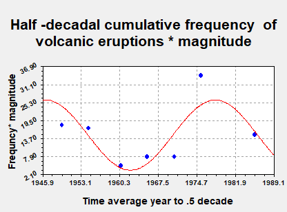
Figure 5

One can also see in this time series the so called 30 year cycle in seismicity characteristic of so many major volcanoes.

However, analysis over a longer timescale to the present day is equally revealing

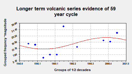
Figure 6

and one can see some evidence of the newly discovered 59 year cycle, see for example McMinn (2011) [22].

Regression factors.

Very interestingly, the regression factors are at their weakest between 1981 -2002. This includes the period in which the famous Mann et al (1998) [23] global warming ‘hockey stick’ was first noted. This was clearly a period in which the QBO did not respond predictably to either solar or anthropogenic input. From the above it can be seen the 30 year seismicity cycle was in decline but the 59 year volcanism cycle had still to build to a maximum.

Clearly the picture is very complicated and it is known that not all volcanism influences the UTLS temperature profile and QBO, see Mehta et al (2015) [24].

For example, Thomas et al (2009) [25] using climate models tried to model the effects of the Mount Pinatubo eruption on the QBO. The effects are complex and result in a strengthened Polar vortex for two winters, AO and NAO ocean effects and mainly stronger effect the second winter after the eruption with some cooling but with warming in the sub –tropics. In my opinion an extrapolation of such observation serves to highlight the possible dangers of would be stratospheric injection style geo-engineering experiments.

Conclusions

Excitingly it has, for perhaps the first time, been possible to employ the QBO to forecast summer season temperatures in the UK. However, the forecast algorithm drifts with time because the QBO is subject to natural drivers from above and below the stratosphere as well as to earth borne anthropogenic drivers.

Taking a naïve approach to results leads to a perceived warming of about .22 C per decade which is consistent with the IPCC’s most recent estimates.

However, taking a more detailed analysis which also appears statistically more reliable leads to a cyclic understanding of recent warming and cooling in terms of linked solar and volcanic activity. Thus the infamous ‘hockey stick’ period of recent warming may well have been created by a rare but coincidental combination of a fall in volcanism and a rise in solar activity the likes of which may only be seen either once every 792 years; 2640 years or 5192 years based on combinations of the three known volcanic, seismic and Gleissberg cycles.

The first two of these take us back to the medieval warm period and Roman warm period consecutively.

At least in North Wales it would appear we have now entered into a cooling phase which could last several decades.

References

1. Graystone, P., 1959: Meteorological office discussion on tropical meteorology. "Met. Mag.", 88, 117.

2. http://www-eaps.mit.edu/faculty/lindzen/qubieoscil.pdf

3. Takahashi M., 1996: Simulation of the stratospheric Quasi-Biennial Oscillation using a general circulation model. "Geophys. Res. Lett.", 23, 661-664.

4. Scaife A.A., et al., 2000: Realistic quasi-biennial oscillations in a simulation of the global climate. "Geophys. Res. Lett.", 27, 3481-3484.

5. Giorgetta M. et al., 2002: Forcing of the quasi-biennial oscillation from a broad spectrum of atmospheric waves. "Geophys. Res. Lett.", 29, 861-864.

6. Ebdon, R.A., 1975: The quasi-biennial oscillation and its association with tropospheric circulation patterns., "Met. Mag.", 104, 282 – 297

7. Baldwin, M. P., and T. J. Dunkerton, 1999: Propagation of the Arctic Oscillation from the stratosphere to the troposphere. J. Geophys Res. Res.,104, 30 937–30 946

8. http://www.drchrisbarnes.co.uk/QBO1.HTML

9. http://yly-mac.gps.caltech.edu/LWS/QBO_solar_Cordero.pdf.

10. http://onlinelibrary.wiley.com/doi/10.1029/96JD02999/abstract

11. https://www.whoi.edu/fileserver.do?id=21466&pt=10&p=17352

12. http://www.ann-geophys.net/33/483/2015/angeo-33-483-2015.pdf

13. http://www.drchrisbarnes.co.uk/Global.htm

14. http://www.cpc.ncep.noaa.gov/products/CDB/Tropics/figt3.gif

15. http://www.esrl.noaa.gov/psd/data/correlation/qbo.data

16. http://www.metoffice.gov.uk/public/weather/climate-anomalies/#?tab=climateAnomalies

17. http://journals.ametsoc.org/doi/abs/10.1175/JCLI-D-14-00224.1

18. http://www.newclimatemodel.com/the-importance-of-solar-cycles-2/.

19. http://journals.ametsoc.org/doi/abs/10.1175/JCLI-D-14-00616.1